Risk of Ruin

Every Forex trader wants to know how risky his strategy is and what’s the chance to lose a part of the account or the whole balance. This chance is called risk of ruin. Since usually Forex traders know their win/loss ratio and the average size of winning and losing positions, calculating the risk of ruin should be relatively easy. Or should it? Unfortunately, it’s not that simple.
Risk of ruin is a known problem in probability theory and to some extent may be solved using the laws and formulas of this theory. Assessing the risk of ruin in Forex is a very complex task that requires a lot of research and calculating powers in exponential dependence on the desirable level of accuracy.
The most popular ways to calculate the risk of ruin of the Forex strategies are two static formulas for fixed position size and fixed fractional position sizing employed currently by many Forex social networks (e.g. FXSTAT, Myfxbook and others). The formulas were presented by D.R. Cox and H.D. Miller in The Theory of Stochastic Processes and are publicly available in various sources (e.g. Minimizing Your Risk of Ruin by David E. Chamness in August 2011 issue of Futures Magazine). They may seem very complex at a first glance, but at a closer look they don’t require any serious amount of calculating powers.
Risk of Ruin with Fixed Position Size
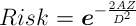
Fixed position size condition suggests that the Forex trader won’t be increasing or decreasing position size with new wins or losses. For example, if one starts with $10,000 account balance and 1 standard lot per position, dropping to $1,000 balance or advancing to $50,000 balance won’t change that 1 lot position volume. The probability to lose a part of balance is exponentially proportional to the standard deviation of the account and is inversely exponentially proportional to the size of this part and the average return per trade. The formula for the risk of ruin is the following:

where:

Example 1:
Risk to lose 10% account balance, considering 2% mean return on a position and a standard deviation of 7%:
Risk = 2.71828 ^ —(2 * 0.02 * 0.1 / 0.07 ^ 2) = 0.442, or 44.2%.
Example 2:
Risk of complete ruin (100% of the account balance), considering 1.5% mean return on a position and a standard deviation of 1%:
Risk = 2.71828 ^ —(2 * 0.015 * 1 / 0.01 ^ 2) = ~5 * 10^—131, or about 0%.
It’s easy to notice that this formula calculates the risk of ruin for the infinite number of trades. According to it, the risk of loss will always be 100% for the system that currently shows negative trade expectancy and will always be close enough to 0 (but not equal to) for the high enough mean return and low enough standard deviation of returns.
Advantages:

Disadvantages:

Risk of Ruin with Fixed Fractional Position Sizing
Unlike the fixed position size model, fixed fractional position sizing implies that a trader is risking a fixed fraction of his account per trade (for example, 1%; the actual value doesn’t really matter here), so the profit is proportional to the account size and the loss is inversely proportional to it. As with the fixed position size, the probability to lose a part of balance is still inversely exponentially proportional to the size of this part. Dependence of the risk on the standard deviation is still positive and on the size of the part is still negative, but its nature becomes more complex. The formula for the risk calculation is the following:

where:

Below are two examples of the risk of ruin calculation using the fixed fractional position sizing model with the same example conditions as for the fixed position size:
Example 1:
Risk = 2.71828 ^ —((2 * 0.02 / 0.07) * (ln(1 — 0.1)/ln(1 — 0.07))) = 0.436, or 43.6%. Obviously, it’s only slightly lower than 44.2% of the fixed position size model.
Example 2:
Since using 100% part of the account balance for the formula would imply that Z = 1, there would be an error in natural logarithm calculation (natural logarithm of 0 is not defined, but it’s an infinitely large negative number). This means that it’s not possible to lose the whole account if the strategy has a positive rate of returns and a fixed fractional position sizing is used:
Risk = 2.71828 ^ —((2 * 0.015 / 0.01) * (ln(1 — 1)/ln(1 — 0.01)))= ~0, or 0%.
Evidently, this formula shows less risk because it assumes a fractional position sizing, which reduces the position size in case of losses, thus reducing the further losses and so on.
Advantages:

Disadvantages:

Gambler’s Ruin Problem Using Markov Chains
The most intuitive method to calculate risk of loss turns out to be the most difficult one in terms of computing. Forex risk of ruin problem can be defined as a particular case of the gambler’s ruin problem, where a trader (player), starting with the initial account balance (stake), has a certain probability to win his average profit amount and a different (or, sometimes, the same) probability to lose his average loss amount. A trader is competing against the market (an infinitely rich adversary) — so only trader can get the account balance ruined; winning condition may be defined as reaching some target balance higher than the starting one.
The formulas and more background research for the simple formulas of risk of loss calculation using this method can be found in Chapter 12 of Introduction to Probability by Charles M. Grinstead, J. Laurie Snell et al.
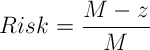
In case, when the average profit equals the average loss, and the probability to lose equals the probability to win, the task of calculation the exact risk of ruin is extremely simple. Starting balance is denoted as z and target balance is denoted as M. The risk of ruining the account before going from z to M then would be:

Example 1:
Starting balance is $10,000 (z). There is 50/50 probability of losing or gaining $1,000 with each trade. Target balance is $20,000 (M):
Risk = (20000 — 10000) / 20000 = 0.5, or 50%.
Obviously enough, the probability of going up from $10,000 to $20,000 is the same as of going down to $0 here.
Probability to win (p) — is a chance to win (end up with profit) one position. It would be very interesting if traders could know their exact probabilities to win a particular trade, but instead the win/loss ratios will be used here. The number of profitable trades divided by the total number of trades will be used as the probability to win. It’s safe to include zero-profit positions here, since it will be compensated by the average win size, it’s just necessary to remember to count such positions when calculating it.
Probability to lose (q) — is a chance to lose (end up with a loss) one position. For the same reasons as above, a plain win/loss ratio is the best number that can be used here. q = Number of losing trades / Total number of trades. Obviously, if 0-profit positions were counted in p calculation, they aren’t to be included here.
If the probability to win a particular trade isn’t the same as to lose it, then a bit more complex formula should be used. Probability of winning an average profitable trade is p, to lose — q (p + q = 1). Then the risk of ruin is calculated as follows:

Example 2:
The starting balance is the same — $10,000 (z), the goal is also the same — $20,000 (M), and the average win/loss is the same $1,000 per trade, but now the probability of winning is 0.55 and the probability of losing is 0.45 (a trading system with 5% edge). To simplify calculations it’s totally safe to divide both the starting and target balances by the average win/loss to get z = 10 and M = 20. The risk of ruin before doubling the balance is calculated as:
Risk = ((0.45 / 0.55) ^ 20 — (0.45 / 0.55) ^ 10) / ((0.45 / 0.55) ^ 20 — 1) = 0.119, or 11.9%.
Evidently, an edge of 5% gives a Forex trader an enormous improvement in reliability of the whole trading system.
In reality, a Forex trading strategy rarely operates with the equal average profit and average loss. The difference in winning and losing position outcomes leads to a much greater complexity in the risk of ruin calculation. It’s pointless to lay out the whole algorithm of calculation in details for this case here. Instead it’s better to provide an overview of the necessary steps, which can be easily reduced to trivial math/coding problems.
Math
The detailed information on the mathematics of the risk of ruin calculation for the general case (different win/loss size and probabilities) can be found in Kevin Brown’s article The Gambler’s Ruin. It’s a superb work that provides an excellent explanation of this problem and the ways of solving it.
The trading process may be represented as a closed-loopMarkov model with one starting state (e.g. $2,500) two end-states — $0 and our target balance (e.g. $5,000). There’s also a number k of transitional states that which depends on the greatest common divisor (GCD) of the average win and the average loss. For example, if the average win is $1,000 and the average loss is $1,500, GCD is $500 and there are 11 transitional states (k = 11), which includes the starting state. The last two transitional states ($4,000 and $4,500) have probability p of reaching the target balance, while the first three states ($500, $1,000 and $1,500) have probability q of ruining the account (reaching $0 balance).
In general, the formula for probability of ruining the whole account before reaching a target balance can be written as follows:

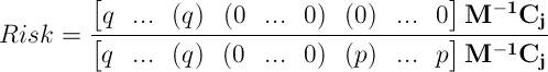
where:

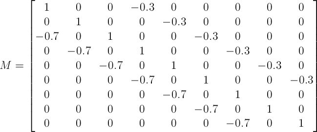
In the above example, the matrix M would look like this:

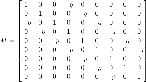
Or, populated with values:

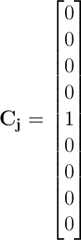
And the vector C_j would look like this:

While matrix/vector multiplication is trivial, inverting a matrix bigger than 3×3 isn’t. The easiest way to find the inverse matrix M^-1 using a computer is LU-decomposition. Using matrix L, it’s possible to solve Ly = I to find y and then to use matrix U to solve Ux = y to find x, which would be M^-1. Multiplying three matrices of the upper part and the three of the lower part of the general formula for probability of ruin is then trivial.
Optimization
The example case is pretty simple, the matrix is only 9×9 — it can be calculated pretty fast without any optimization. But what if the GCD of the strategy is $1? For example, if the average loss is $1,113 and the average profit is $1,109, the GCD is $1. With $2,500 starting balance and $5,000 target, that’s 4,999×4,999 matrix — that will require a lot of memory and time to calculate. The best time of computing this risk of ruin without any optimization is O(k^2.376) and in general it requires at least k×k memory.
Firstly, it’s important to keep the M^-1 matrix as small as possible. Optimally k, should be less than 500, if the aim is to solve this problem in reasonable time (several seconds).
Secondly, the required memory can be reduced significantly: the losing vector can be stored inside the total vector (it’s known where the q‘s in the losing vector stop and the 0’s begin), and the results of the LU decomposition can be stored inside the main matrix (M; it won’t be needed it after decomposing).
Thirdly, both Ly = I and Ux = y can be solved for one column (jth), instead of the whole k×k matrix. That same column will also be a result of multiplication with C_j (if the whole k×k matrix is calculated and then multiplied by C_j, the result will also be jth column of the matrix, because of all the zeros in C_j).
Lastly, it’s possible to calculate the product of the losing vector with the jth column and the product of the total vector with that column simultaneously, as the first loss step iterations will be the same during that calculation and other iterations aren’t needed in case of the losing vector.
Implementation
Example PHP code that uses the above algorithm to find the risk of ruin for the earlier example:

	/*
	  Starting balance:      $2,500.00
	  Target balance:        $5,000.00
	  Avg. losing trade:     $1,500.00
	  Avg. profitable trade: $1,000.00
	  Loss probability:      30%
	  Win probability:       70%
	*/
 
	$begin_state = 5;
	$N = 9;
	$loss_step = 3;
	$win_step = 2;
	$q = 0.3;
	$p = 0.7;
 
	// Filling Cj
	for ($i = 0; $i < $N; $i++)
		if ($i == $begin_state - 1) $unitary_vector[$i] = 1;
		else $unitary_vector[$i] = 0;
 
	// Filling loss vector and total vector. Loss vector is actually a part of total vector
	for ($i = 0; $i < $N; $i++)
		if (($i - $loss_step) < 0) $total_vector[$i] = $q;
		else if (($i + $win_step) >= $N) $total_vector[$i] = $p;
		else $total_vector[$i] = 0;
 
	// Filling the main matrix
	for ($i = 0; $i < $N; $i++)
		for ($j = 0; $j < $N; $j++)
			if ($i == $j) $a[$i][$j] = 1; // Main diagonal is always 1
			else if ($j == $i + $loss_step) $a[$i][$j] = -$q; // Elements to the above the main diagonal are about losing
			else if ($j == $i - $win_step) $a[$i][$j] = -$p; // Elements to the below the main diagonal are about winning
			else $a[$i][$j] = 0;
 
	// LU Decomposition
	for ($i = 0; $i < $N; $i++)
	{
		for ($j = $i; $j < min($N, $i + $loss_step); $j++) // U
			for ($k = 0; $k <= $i - 1; $k++)
				$a[$i][$j] -= $a[$i][$k] * $a[$k][$j];
 
		for ($j = $i + 1; $j <= min($i + $win_step, $N - 1); $j++) // L
		{
			for ($k = 0; $k <= $i - 1; $k++)
				$a[$j][$i] -= $a[$j][$k] * $a[$k][$i];
			$a[$j][$i] /= $a[$i][$i];
		}
	}
 
	// Solving Ly = I for one column (unitary_vector) that is equal to Cj of the Gambler's Ruin formula
	// The resulting y will be also stored in unitary_vector
	for ($i = $begin_state; $i < $N; $i++) // Start from begin_state because all X's before 1 in the unitary_vector will always be 0
	{
		$sum = 0;
		for ($j = 0; $j <= $i - 1; $j++)
			$sum -= $a[$i][$j] * $unitary_vector[$j];
 
		$unitary_vector[$i] = $unitary_vector[$i] + $sum;
	}
 
	// Solving Ux = y for one column that was calculated in Ly = I
	// The resulting x will be stored in unitary_vector
	for ($i = $N - 1; $i >= 0; $i--)
	{
		$sum = 0;
		for ($j = $N - 1; $j > $i; $j--)
			$sum -= $a[$i][$j] * $unitary_vector[$j];
 
		$unitary_vector[$i] = ($unitary_vector[$i] + $sum) / $a[$i][$i];
	}
 
	// Multiplying total_vector and its losing part by the resulting unitary_vector.
	$loss = 0;
	$total = 0;
	for ($i = 0; $i < $N; $i++)
	{
		$product = $total_vector[$i] * $unitary_vector[$i];
		if (($i - $loss_step) < 0) $loss += $product;
		$total += $product;
	}
	$probability = $loss / $total;
	echo "Loss: $loss 
";
	echo "Total: $total 
";
	echo "Probability: $probability 
";
?>

= $N) $total_vector[$i] = $p;
else $total_vector[$i] = 0;

// Filling the main matrix
for ($i = 0; $i < $N; $i++) for ($j = 0; $j < $N; $j++) if ($i == $j) $a[$i][$j] = 1; // Main diagonal is always 1 else if ($j == $i + $loss_step) $a[$i][$j] = -$q; // Elements to the above the main diagonal are about losing else if ($j == $i - $win_step) $a[$i][$j] = -$p; // Elements to the below the main diagonal are about winning else $a[$i][$j] = 0; // LU Decomposition for ($i = 0; $i < $N; $i++) { for ($j = $i; $j < min($N, $i + $loss_step); $j++) // U for ($k = 0; $k <= $i - 1; $k++) $a[$i][$j] -= $a[$i][$k] * $a[$k][$j]; for ($j = $i + 1; $j <= min($i + $win_step, $N - 1); $j++) // L { for ($k = 0; $k <= $i - 1; $k++) $a[$j][$i] -= $a[$j][$k] * $a[$k][$i]; $a[$j][$i] /= $a[$i][$i]; } } // Solving Ly = I for one column (unitary_vector) that is equal to Cj of the Gambler's Ruin formula // The resulting y will be also stored in unitary_vector for ($i = $begin_state; $i < $N; $i++) // Start from begin_state because all X's before 1 in the unitary_vector will always be 0 { $sum = 0; for ($j = 0; $j <= $i - 1; $j++) $sum -= $a[$i][$j] * $unitary_vector[$j]; $unitary_vector[$i] = $unitary_vector[$i] + $sum; } // Solving Ux = y for one column that was calculated in Ly = I // The resulting x will be stored in unitary_vector for ($i = $N - 1; $i >= 0; $i–)
{
$sum = 0;
for ($j = $N – 1; $j > $i; $j–)
$sum -= $a[$i][$j] * $unitary_vector[$j];

$unitary_vector[$i] = ($unitary_vector[$i] + $sum) / $a[$i][$i];
}

// Multiplying total_vector and its losing part by the resulting unitary_vector.
$loss = 0;
$total = 0;
for ($i = 0; $i < $N; $i++) { $product = $total_vector[$i] * $unitary_vector[$i]; if (($i - $loss_step) < 0) $loss += $product; $total += $product; } $probability = $loss / $total; echo "Loss: $loss
“;
echo “Total: $total
“;
echo “Probability: $probability
“;
?>

The output would be:
Loss: 0.25755603952
Total: 1
Probability: 0.25755603952
So the risk to ruin the whole account before doubling it is about 25.8% for this example.
But what if k is getting to big? In this case, mathematical rounding should be applied to loss step, win step and both starting and target balances, virtually truncating some of the last digits. Additionally, the target balance can be reduced. The first method influences the accuracy, but its effect is less important the bigger is the difference between the average loss and the average profit.
Advantages

Disadvantages

Conclusion
None of the described methods is perfect. Each should be used when it fits the parameters of the Forex trading strategy:

Whichever method is selected, it’s important to remember that the resulting risk value shouldn’t be taken too seriously by its own. Its main purpose is in comparing different strategies or the effect of the changes applied to one trading strategy. Relying on the calculated risk value as the real measure of strategy riskiness can lead to unexpected but horrible consequences.
Note: it’s possible to calculate all three types of risk of ruin by using the Forex Report Analysis Tool. Perhaps the only free online tool that offers such functionality.

If you have any questions or commentaries regarding the assessment of the risk of ruin in Forex trading, please feel free to post them using the form below.